Chapter 1: How Demand Works in Education
Unit I: Foundations – Supply, demand, and market basics

Every year starting from March, (though some get decisions even earlier because of early decision or early action) a sort of ritual unfolds in households across the country. Families hover over laptops or family computers, waiting for admissions decisions from a handful or even a dozen or more universities that the graduating high school senior applied to. Some even record their reactions to share on social media, sharing with the dozens or the thousands watching the joy of an acceptance or disappointment of a rejection. When I was a student, these replies would arrive by mail (i.e. the postal worker delivering it to the physical mailbox), and you wouldn’t even need to open the envelope to know if it was good news or bad news. If someone got an acceptance, it would be a large colorful envelope, and often quite a thick package with all the information needed. If it was a waitlist or rejection, what was recieved was just a simple plain envelope, no bells or whistles. These days everything starts with admissions portals and emails. Once the decisions come in, and with FAFSA filed, next come the financial aid packages and comparisons there. Families then weigh rankings versus cost versus distance from home, gut feeling against career outcomes data. Family connections. Some students apply to twenty schools. Some apply to three. Some do not apply at all, because they already know the numbers do not work and are planning on going to community college or straight to work.
All of these household choices together form the demand for higher education. All these considerations are part of the demand function for a four-year undergraduate degree (or even a two-year associate one).
Not all families would like to think of it as such. For some students getting into a dream school is enough to override almost all logic. But even then, that strong preference for a school, is still a function of their individual demand curve. It is what an economist calls a determinant of demand.
What demand actually means
In everyday speech, demand means something like desire or need for something. This could be a statement like “there is high demand for good food” or “I demand an explanation.” In economics, the word has a more precise meaning. Demand is not just simply wanting something. It is wanting it and being willing and able to pay for it.
This distinction matters. Consider two students. Sarah has been dreaming of attending a particular private university, Northwood University, for the last couple of years, and her family is able to afford it. She visited the campus, attended several information session, and ranks it first on her priority list. She may have even applied early decision. The other, Jamie, would love to go there, but has never seriously considered it. The tuition is twice what her family could possibly manage, even accounting for financial aid, and there is no realistic path for Jamie to to afford attending Northwood.
At the current tuition rates and financial aid on offer, only one of these students is part of the demand for this institution. It is not the one with the stronger desire to go there, but rather the one who has the ability and willingness to actually pay the tuition.
When the admissions office (or the consultant) is analyzing “how much demand do we have?” they are not really considering how many people would like to attend ignoring price altogether. They are estimating how many people, at this given tuition and financial aid levels, will pay a deposit, pay tuition and enroll at the university. That is how many new students will be there at the beginning of the Fall semester.
The quantity demanded of a good, in this case a place at a less-selective four-year university, is the number of buyers (consumers) are willing and able to purchase at a specific price, holding everything else constant. This last condition, ceteris paribus or all else equal, is an important concept in microeconomics. It is a simplification, part of our economic modeling, but it means we are asking a specific question. This lets us ask the question, for example, how much would a price change affect the quantity of goods or services buyers are willing to buy. For our current example, that is to say, if tuition was lowered or more financial aid was offered, would there be more students willing to apply and enroll at Northwood? And all of this is considered while assuming everything else stays the same, i.e. families are not wealthier, or there are no new colleges opening or closing nearby. We hold those things fixed so we can see the effect of the price change clearly.
The law of demand and the demand curve
The law of demand is not necessarily the same as law of physics – it’s not gravity or electromagnetism. Yet it is quite robust, one of the most consistent findings in all of economics. Simply put, the law of demand states that when the price of something rises, the quantity demanded falls. And when the price falls, the quantity demanded rises. It holds up across markets, goods and services, and time. Often you will find textbooks that mention a few exceptions, Giffen goods and Veblen goods are brought up as examples, but more often than not, these exceptions are violating the ceteris paribus assumption and are being driven by changes in other factors.
The law of demand is intuitively simple when you consider it.
Consider affordability. Higher prices put the good or service out of reach for some buyers who were previously just able to buy it. Suppose a public state university announces a thirty percent decrease in tuition. A family with several children who were stretched financially and not able to afford the tuition at this public four year institution will recalculate and decide that they are able to afford it. Now they are able and willing to send all their childen to college. So quantity demanded increases. These folks who might not have gone to college can now choose to attend. We call this an income effect. By making college (a major expense for a family with multiple children) cheaper, it allows a family to afford more of everything, including more college for the rest of the family.
The second is substitution. When the price of Riverdale University decreases, it begins to look more attractive by comparison. A prospective student who might have paid $38,000 a year in tuition for a private school may look at things very differently now that Riverview lowered tuition from $24,000 to $16,000 a year. The quality of the private school vs public school has not necessarily changed. But the relative price has, so the public option could be the more desirable option now since it is more cost-effective.
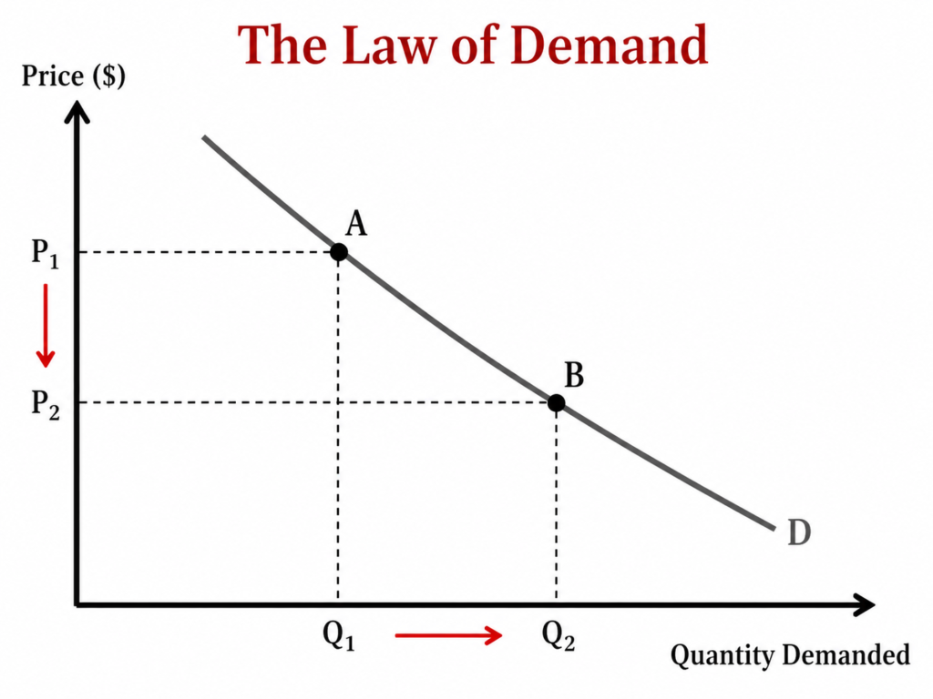
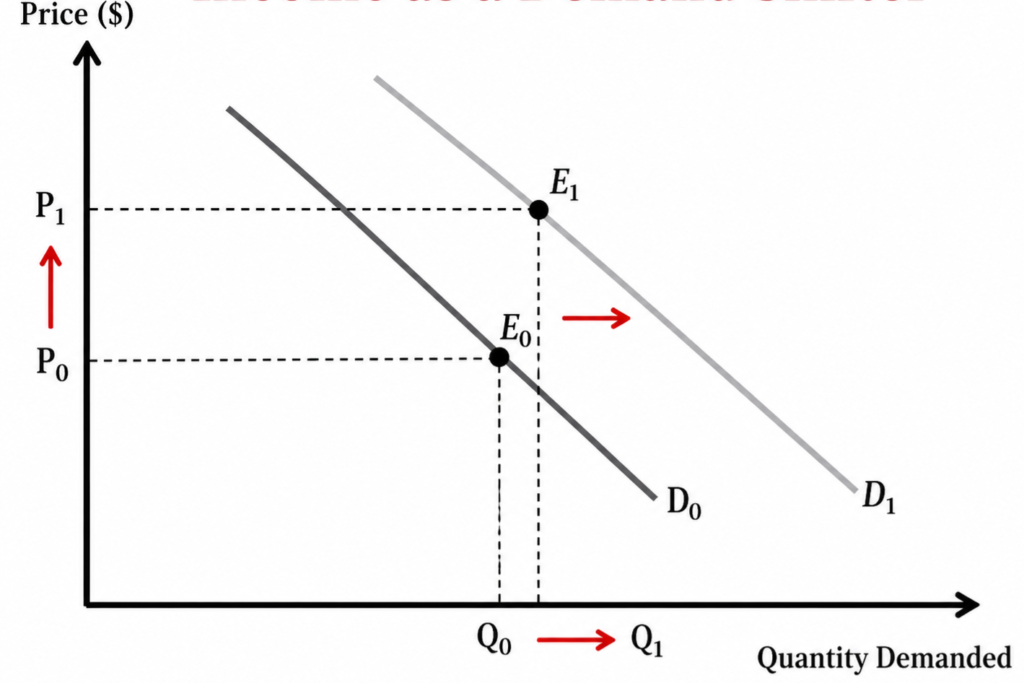
We represent this relationship graphically with a demand curve. This is a line, typically drawn sloping downward from left to right, that shows how much of a good buyers would demand at each possible price. Price is on the vertical axis, and quantity demanded is on the horizontal axis. Moving down the curve corresponds to a lower price and higher quantity demanded. Moving up corresponds to a higher price and lower quantity demanded.
This can also shown in the form of a demand schedule, which is simply the same information in table form. They are two ways of representing the same underlying relationship.
A movement along the curve versus a shift of the curve
One of the things I have found students have a difficulty differentiating is a change in price versus a change in the other factors that affect demand. It is important so let us spend some time on this. When the price of a good or service changes, there is a corresponding change in the quantity demanded. This is called a move along the demand curve. The existing and same demand curve. We move from one point on the curve to another point on the same curve. The curve itself does not move. Consider the original demand curve D0. When Riverdale lowers the price from $24,000 (P1) to $16,000 (P2), the quantity demanded increases from Q1 to Q2. There is a movement along the demand curve from A to B.
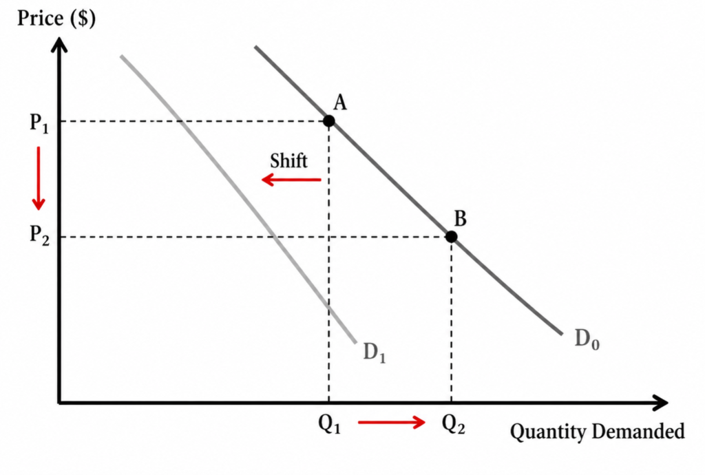
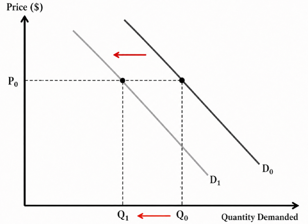
When something other than price changes – income, demographics, tastes, the price of a substitute, buyer expectations (we will discuss these determinants below in more details), the entire demand curve shifts. For every price the quantity demanded has now changed, and we have a new demand curve D1. In our graph, one of those other determinants have led to a deacrease in demand.
Why does this matter? Because confusing the two will lead to the wrong conclusion about what is happening in a market. Here is a hypothetical scenario to emphasize why the distinction is important.. Imagine a small liberal arts college in the Midwest, Ridgeview College, that has seen enrollment decline by thirty percent over five years. The president and the board are sitting together, trying to diagnose the issue. There are two explanations being discussed at the board meeting.
Option 1: Ridgeview raised tuition aggressively over the last 5 years while other nearby colleges have not. Some prospective students who might have chosen Ridgeview instead chose cheaper options elsewhere. Enrollment fell because of a movement along the demand curve, higher prices, lower quantity demanded, and the college moved up along the same demand curve.
Option 2: The regional population of 18-year-olds has fallen significantly as there has been significant migration out of state along with fewer children being born from the mid-2000s. So the demand for college in the region has dropped across every institution, regardless of price. The demand curve itself has shifted left.
Now consider the two options. Very different things are happening in each of these cases, and the solutions that the Ridgeview College needs to pursue in response is very different. And you cannot design the right response until you know which one is correct.
What shifts the demand curve: the five determinants
Economists identify five non-price factors that can shift demand, the determinants.
1. Prices of related goods
Goods and services can be related in two ways: as substitutes or as complements.
Substitutes are alternatives. These are goods or services you might buy instead of the original. For a student choosing between a four-year public university like Riverdale University and a private liberal arts college like Ridgeview College, these institutions are substitutes. When the public school tuition falls, or when the public colleges make it easier to apply, or offer additional majors, some students who might otherwise have enrolled the private liberal arts college might choose to go the public route. The demand for the private Ridgeview College shifts left – not because anything changed at the liberal arts institution, but because the substitute (public university) became more attractive.
Similarly when for-profit online programs expanded aggressively in the 2000s, driven by the rise of the internet, offering flexible schedules, distance-learning, and lower upfront costs, they drew students away from traditional regional universities. The four-year regional colleges and universities had not done anything wrong. A substitute had gotten cheaper and more accessible, and demand shifted accordingly.
Complements are goods that tend to be consumed together. So, a fall in the price of one raises demand for the other. Student off-campus housing and college enrollment are a kind of complement in this sense. A college that sees a significant increase in enrollment will see an increase in the demand for housing in nearby neighborhoods. This can be seen clearly in small collegetowns during the COVID pandemic when colleges sent students home and collegetowns saw empty rental units and declining rents.
Laptops and internet access are also complements for online education. As broadband access expanded through rural areas in the 2010s, demand for online degree programs grew in these areas, not because those programs improved, but because a complement got cheaper and more widely available.
2. Income
For most goods, an increase in income raises demand. Economists call these normal goods. College enrollment generally behaves this way, i.e. in periods of economic growth, more families have additional income and thus enrollment at four-year institutions, and enrollment at private universities tends to rise. This is an increase in demand, we show this as a rightward shift of the demand curve.
The 2008 financial crisis offered a natural experiment in reverse. Household incomes fell sharply across a large fraction of American families. As expected, some students who had expected to attend four-year schools shifted to community colleges. Some who had expected to live on campus commuted from home instead. Some delayed enrollment altogether. And we can demonstrate this with a leftward shift in demand caused by a shock to household income and resources.
But here is where it gets interesting. Not every type of institution behaves like a normal good. Some exhibit the characteristics of inferior goods. These are goods or services for which demand actually rises when income falls, because they serve as a cheaper alternative to something else.
Consider the effects of the 2008 financial crisis and the recession that followed. Community colleges saw enrollment increase as family incomes declined. Some of those students were always planning to attend community college. But some students who had planned on going to four-year colleges changed plans and with lower family income, chose to enroll in community college. This is not a reflection on quality, but a description of how demand for it responds to income. Other popular things are inferior goods – public transportation, ramen, public elementary schools. Wealthy households (or households whose incomes increase) will demand less public transportation and less public elementary schools and instead buy cars and send their children to private elementary schools.
The distinction matters for institutions thinking about their financial resilience during turbulent times. A university whose students are predominantly from high-income households may find enrollment relatively stable during a recession, because those families have enough buffer to absorb income shocks. However, a private university serving a wider student body and with students enrolling from all walks of life will find that its demand will decrease when the economy is in trouble.
3. Tastes and preferences
Tastes are the most slippery of the five shifters, but also one of the most powerful. They capture everything that shapes how buyers value a good that is not captured by price or income — cultural norms, information, peer effects, changing ideas about what constitutes a good life.
For higher education, one of the most consequential taste shifts of the last half-century has been the slow hardening of the belief that a four-year college degree is the default path to a middle-class life. This was not always the norm. In the 1960s and 1970s, a much smaller fraction of Americans attended college, and most decent jobs did not require a degree. As the wage premium for college graduates grew — the so-called college premium, the gap in lifetime earnings between degree-holders and non-degree-holders — attitudes shifted. College became not just an option but an expectation. Demand for higher education rose, at every price level, across the income distribution.
That taste shift is now being tested from the other direction. A growing share of prospective students and their families — especially after years of headlines about student debt, job market disruption, and the success of high-profile non-graduates — are questioning whether the four-year degree is automatically worth the cost. Coding bootcamps, apprenticeship programs, and employer-sponsored credentials have become culturally legitimate in a way they were not a decade ago. If this represents a genuine shift in tastes, rather than a temporary fluctuation, the demand curve for traditional higher education could shift left over time — not because of price, and not because of demographics, but because the underlying valuation of the good has changed.
Institutions are acutely aware of this. It is why so many universities now invest heavily in outcome data — placement rates, median salaries of graduates by major — and publish them prominently. They are trying to maintain demand by reinforcing the taste for their product. In a market where preferences are shifting, information can do what price discounts alone cannot.
4. Population and demographics
This is the bluntest of the five shifters, and right now the most consequential one for American higher education.
The number of potential college students at any given time is largely determined by birth rates eighteen years earlier. You can market aggressively, offer generous aid, build beautiful facilities, and hire exceptional faculty — but you cannot recruit students who were never born. The size of the college-age population is, to a significant degree, simply a given for any institution operating in the present.
Here is the problem. Birth rates in the United States fell sharply starting around 2008, during and after the financial crisis. Those smaller cohorts of children are now turning eighteen. The WICHE projections show a clear picture: the number of high school graduates, which is the primary feeder pool for college enrollment, will begin declining meaningfully in many states around 2025 and will fall more sharply in some regions through the late 2020s and into the 2030s.
This is a simultaneous, multi-year leftward shift in the demand curve for college seats — not a movement along the curve in response to a price change, but a structural reduction in the size of the buyer pool. It is happening regardless of what institutions charge, what programs they offer, or how well they market themselves.
The geographic distribution of this shift matters enormously. The demographic decline is most severe in the Northeast and Midwest — regions that also happen to have the highest concentration of small private colleges already operating with thin margins. A college in rural Ohio or Vermont that has maintained enrollment in recent years partly by drawing from a regional applicant pool that is about to shrink significantly faces a very different situation than a nationally recognized research university that draws applicants from across the country and abroad.
International students are one partial offset. If domestic demand declines, institutions have increasingly sought to backfill enrollment with international applicants, for whom geographic proximity matters less and the appeal of a US degree remains strong. This works, up to a point. But it introduces its own volatility — international enrollment is sensitive to visa policy, exchange rates, geopolitical relationships, and competition from universities in Canada, the UK, and Australia, all of which have been actively recruiting the same pool.
5. Buyer expectations
The last shifter is the most forward-looking. Demand today is shaped not just by present conditions but by what buyers expect the future to look like.
Consider the decision to enroll in a nursing program. If prospective students expect strong job growth in healthcare over the next decade — and the projections broadly support this — demand for nursing programs will be high even if the programs are expensive and demanding. The expected future return justifies the present cost.
Now consider a prospective law student in the early 2010s, watching the job market for new law school graduates deteriorate sharply and reports about high debt loads and underemployment spread across legal publications and mainstream media. Applications to law schools fell dramatically — not because tuition rose sharply, not because the population of potential applicants shrank, but because buyers updated their expectations about the return to the credential. The demand curve for law school seats shifted left, driven almost entirely by changed expectations.
The same dynamic operates at the level of the institution, not just the program. A university that suffers a highly publicized scandal — a major Title IX failure, an accreditation warning, a fraud investigation — may see its demand curve shift left as prospective students update their expectations about what attending that institution will mean for their outcomes and reputation. Conversely, a university that sees its rankings improve significantly, or lands a high-profile research grant, or has a prominent alumnus make news, may see demand shift right as expectations about quality and prestige are revised upward.
Expectations are self-fulfilling in a way that makes them particularly powerful in higher education. If students expect a degree from Institution A to be valued by employers, they will seek that degree more intensely, which increases selectivity, which signals quality, which reinforces the employer valuation. The feedback loop between expectations and outcomes is one of the reasons that reputational rankings are so sticky, and why it is so hard for institutions to climb them once they have settled.
Elasticity: how much does quantity actually respond to price?
Knowing that higher prices reduce quantity demanded is useful. Knowing how much quantity responds is far more useful. This is what economists measure with elasticity — specifically, the price elasticity of demand.
The formula is straightforward: divide the percentage change in quantity demanded by the percentage change in price. If tuition at a university rises by 10% and applications fall by 5%, the price elasticity of demand is -0.5. If they fall by 20%, it is -2.0. The sign is always negative (higher price, lower quantity), so economists often drop it and refer to the magnitude.
When the magnitude is greater than one, demand is elastic — quantity is relatively responsive to price. When it is less than one, demand is inelastic — quantity does not respond much. When it is exactly one, we call it unit elastic.
The intuitive question is: what determines whether demand is elastic or inelastic in higher education?
The availability of substitutes is the most important factor. If a prospective student views several institutions as genuinely interchangeable — similar programs, similar outcomes, similar culture, convenient to home — then a price increase at one of them will send her fairly easily to the others. Demand is elastic. If she has a highly specific reason for wanting one particular institution — a program that only exists there, a location that works for a family situation that cannot change, a relationship with a faculty member who is doing work she wants to be part of — then a price increase will not move her much. Demand is inelastic.
This is why elite universities occupy such a different pricing environment than regional institutions. Harvard’s price elasticity of demand is approximately zero. There is no substitute for Harvard in the minds of the students and families who want it most. The institution can raise tuition — and does, year after year — without meaningfully reducing its applicant pool, because the people applying are not cross-shopping with other options in any normal consumer sense.
A regional public university in a state with four other public options, serving students who are largely in-state and cost-conscious, faces a very different situation. A meaningful tuition increase will cause some students to shift to community college, some to a neighboring state school, and some to delay enrollment. The substitutes are real and accessible. Demand is elastic.
The proportion of income or budget devoted to the purchase is a second determinant. When a good accounts for a large share of a buyer’s total budget, they tend to be more price-sensitive — a price change represents a large absolute dollar shift in their situation. College tuition is one of the largest single expenditures many families ever make. This tends to push demand toward elastic, particularly for families with limited financial cushion. For a family comfortably in the top income quintile, a $3,000 tuition increase is an annoyance. For a family at the median, it may be the difference between enrolling and not.
Time horizon also matters. In the short run, demand for a specific institution can be quite inelastic — a student who has already been admitted, visited campus, and committed emotionally to attending is not going to walk away easily over a moderate price increase announced in April. In the longer run, reputation and price signals shape the pool of students who apply in the first place, and the elasticity over multi-year periods is considerably higher. Institutions that have raised prices aggressively over a decade often find that the composition of their applicant pool has quietly shifted — they are drawing from a wealthier and narrower demographic, not because that was the plan, but because the economics selected for it.
Two hypothetical institutions, one demand lesson
Let me illustrate the full framework with a hypothetical scenario that brings together several of the concepts above.
Imagine two institutions in the same mid-sized American city. Westfield University is a mid-tier private with a strong regional reputation, a wide range of undergraduate programs, and a student body drawn primarily from the surrounding three states. Municipal Community College sits across town, offering two-year degrees, certificates, and a well-used transfer pathway to the state university system.
Westfield’s tuition is $42,000 per year. Municipal’s is $6,000.
Now the state legislature, facing a budget surplus, announces a significant expansion of Pell Grant eligibility and a new state grant program that covers full tuition at community colleges for students whose family income is below $75,000.
Walk through the demand effects.
For Municipal, this is a direct reduction in the effective price for a large share of its prospective students. The quantity demanded at every income level increases. The demand curve shifts right — more students want to attend because the net cost has fallen dramatically. Municipal needs to think seriously about capacity.
For Westfield, the effects are more complicated. Some students who had been stretching to afford Westfield may now find that Municipal — newly free for them — represents a much better deal, particularly if their primary goal is a credential for the job market rather than the four-year residential experience. These students shift their demand from Westfield to Municipal. Westfield’s demand curve shifts left at the lower end of its income distribution.
But a different group of students — those who had been planning to attend Municipal as a cost-saving first step before transferring to a four-year school — may now bypass Municipal and go straight to Westfield, since the financial calculus has shifted. This pulls demand toward Westfield among a segment that would previously have been Municipal’s.
On net, Westfield probably loses some demand, particularly among its most price-sensitive applicants. What should it do? It could increase its own financial aid to compete more directly with the newly strengthened community college option — a response along the demand curve. Or it could invest in differentiating itself more sharply from the community college substitute — better career outcomes, more distinctive programs, a stronger residential experience — a strategy aimed at making the demand curve less elastic by reducing the perceived substitutability. Both responses are legitimate. The demand framework helps identify which lever is which.
The demand side of the enrollment cliff
Let me close this chapter with something that is not hypothetical at all.
The United States is in the early stages of a demographic shift that will be one of the most consequential forces in American higher education over the next fifteen years. Birth rates fell sharply after the 2008 financial crisis and have not fully recovered. Those smaller birth cohorts are now approaching college age. The WICHE projections show the number of high school graduates beginning to decline meaningfully in many states starting around 2025, with the steepest drops in the late 2020s and early 2030s — disproportionately concentrated in the Northeast and Midwest.
For higher education, this is a sustained leftward shift in the aggregate demand curve for college seats. Not a movement along the curve driven by price. A structural contraction in the size of the buyer pool.
The arithmetic is unforgiving. If a regional private college currently enrolls 1,200 first-year students and draws from a pool of roughly 18,000 high school graduates in its primary recruitment region, and that pool shrinks by 20% over the next decade, the college needs to either reach further geographically, convert a higher fraction of its existing pool, or accept that its incoming class will be smaller. Usually some combination of all three. And if the college was already operating at or near the financial breakeven point for its current enrollment — as many small private institutions are — any of these outcomes creates real strain.
The demand curve does not care about an institution’s history, its mission, or how beloved it is by its alumni. It reflects the decisions of actual people with actual resources in an actual economy. When those people are fewer, something has to give — prices, capacity, programs, or the institution itself.
Understanding the sources of demand for education — and the forces that shift that demand — is not just an academic exercise. It is a framework for understanding which institutions are vulnerable, which are resilient, and what the policy levers are for an industry facing a structural shock it cannot price its way out of.
The rest of this unit turns to supply. Which has its own set of constraints, its own set of rigidities, and its own uncomfortable reckoning with the same demographic reality.